Analysis of Proteomics Data
Tom Radcliffe
Predictive Patterns Software Inc.
http://www.improvedoutcomes.com
Summary
This case study involves a
blinded proteomics dataset. It is based on a study of data supplied
for a proof-of-concept analysis, but uses simulated data. It details
various strategies for using GeneLinker Platinum to solve a difficult
classification problem. However, it includes many examples of
GeneLinker Gold features used to explore the data and devise a strategy for
analysis.
It also demonstrates the
power of multiple classifications: even in cases where no single
classifier was able to call every test sample, using multiple
classifiers enabled the almost perfect classification of unknowns.
Description of Data
The data consist of two
files of mass spec data:
- TrainingData.csv
- TestData.csv
The TrainingData file
consists of samples that are known to belong to one of four groups.
There is a separate variable file that contains a single column
giving the group for each of these samples.
There are four groups: A,
B, C and D labeled in the last column of the training file, as
follows:
- A: 78 samples
- B: 83 samples
- C: 83 samples
- D: 81 samples
The data for each sample
are 570 channel values that have been extracted from the original
spectra.
TestData.csv contains 60
samples of unknown group. Part of this study will show how
confidence in classification can be high even when the test samples
are truly of unknown group.
Classification Task
The classification task is
to find features (channel values) and classifiers (ANNs, IBIS or
others) that discriminate between groups reliably.
Rather than try to develop
a single classifier that will distinguish all-from-all, it is often
simpler to "divide and conquer" by first finding a
classifier that distinguishes one group from all the others and then
repeating this strategy until only one group is left.
This report focuses on D
vs. ABC. The best classifier system found has good (>99%)
accuracy on a test data set split off from the training samples
provided, and gives a self-consistent classification of the blinded
test data.
Preliminaries
The data were imported
into GeneLinkerTM Platinum and given an initial high-level
analysis using Gold-level functionality to determine their general
characteristics. Samples were labeled S1 through S325.
Preliminary analysis found heterogeneity, redundancy and outlier
issues.
Heterogeneity
The data values range from
about -10 to +100. Histogramming shows the usual log-normal
distribution characteristic of much biological and chemical data (for
the purposes of this study data were in fact generated to ensure this
was the case, including the dual Gaussian structure shown below, and
the outliers discussed in the next section.) Negative values were
removed and replaced with the median of their channel. Channels with
more than 30 negative values (10%) were deleted from the dataset.
This resulted in a reduction in the number of channels from 572 to
332. The data were then normalized by taking log10, and the
resulting histogram is as shown in Figure 1.
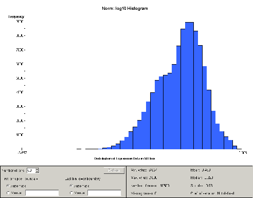
Figure 1: Histogram of all samples after log normalization
As can be seen, the data
appear to contain two distinct but overlapping populations.
Splitting the dataset into four chunks, one for each group and
repeating this preliminary
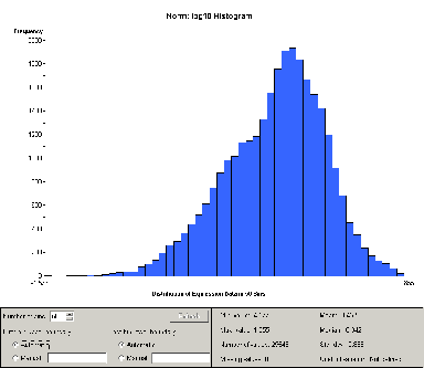
Figure 2: Histogram of just Group B samples after log normalization
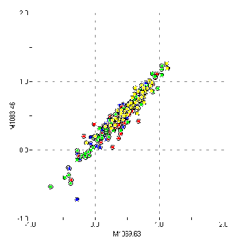
Figure 3: Correlation between adjacent entries
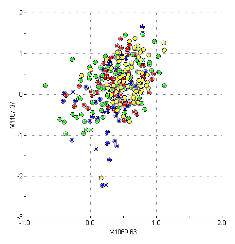
Figure 4: Uncorrelated columns separated by 100 daltons
analysis on each group
reveals that this heterogeneous structure is present on all classes
individually. For example, the histogram for Group B is shown in
figure 2.
This is important because
it means there is gross structure in the data that is unrelated to
the grouping variable, and therefore may confound any attempt at
classification.
Redundancy
A second type of
preliminary analysis was also performed. Pairs of columns were
examined for correlation using GeneLinker's Scatter Plot
functionality. A few random pairs were selected from the whole of
the data.
It was immediately
observed that adjacent or nearby columns were highly correlated, as
shown in Figure 3. More distant columns were not significantly
correlated, as shown in Figure 4.
Mass spec systems
typically have strong correlations between adjacent channels due to
finite resolution—a peak is naturally extended over many
channels. Therefore the correlation between nearby columns in these
data strongly suggests they are channel (intensity) data rather than
peak (area) data. On this basis the individual entries are referred
to in this report as “channels” rather than “peaks”.
This is significant for
subsequent data analysis because it means the data, already fairly
sparse, are also significantly redundant, and some data mining
methods will pick up several adjacent columns as “significant”
when in reality only one of them carries unique information—the
rest will just be repeating the same information. Therefore
post-processing of results may yield smaller sets of equally good
discriminators when these redundant columns are removed
Outliers
A final aspect of the data
that was uncovered in the preliminary analysis was the presence of
outliers in Group C. PCA analysis as shown in Figure 5, revealed a
“blob” of samples far from everything else. The 19
samples in this blob were culled from the data prior to further
analysis, reducing the number of Group C samples to 64 from 83.
There are three samples in this culled set that are perhaps
questionable (the ones in the upper right corner of the red overlay).
However, their presence or absence does not make a difference to the
results of analysis, which were ultimately verified on the whole
dataset.
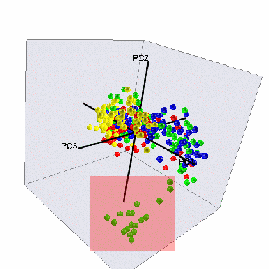
Figure 5: Group C outliers culled from the dataset on the basis of
PCA as shown
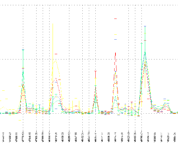
Figure 6: Partial plot of un-normalized merged data. Error bars
show standard deviation.
Data Quality
To assess data quality,
samples in each group were merged and the resulting values plotted.
A detail from this plot is shown in Figure 6.
Two things are immediately
apparent: the between-group variation is much smaller than the
standard deviation within each group, and adjacent channels really do
frequently contain redundant information. The large within-group
variation compared to the between-group variation makes the posed
discrimination tasks challenging.
Splitting
To use the supervised
learning capability of GeneLinker™ Platinum effectively the
data from Train.csv were split into a training and test set that the
known groups of the test set could be used to evaluate the quality of
classification. The test set comprised approximately 30% of the
data, randomly selected across all four groups.
Splitting of data files
and generation of variable files was done outside of GeneLinker™
using Perl scripts. Splitting and variable generation functionality
will be added to GeneLinker™ in a release later this year.
Summary
The purpose of the
foregoing is to demonstrate a few of the ways you can use the
capabilities of GeneLinker to examine the gross features of your
data. There is no more important step in data analysis: the most
sophisticated analysis algorithm will produce bad results when fed
bad data.
Outline of Analysis
All classification tasks
were approached in a similar way. The data were log-normalized as
described above, and several parallel approaches were used for
feature selection:
Each of these approaches
was used to find a small set of channels that were promising
candidates to perform the classification task. One or more
committees of neural networks were then trained in these candidate
channels, and the quality of classification was evaluated using the
fraction of the data held out from the original training dataset.
Note that evaluation was used sparingly, as over-use of a validation
set can effectively turn it into a secondary training set, with the
data analyst serving as part of the training algorithm.
Once reasonable
performance was achieved on features selected by each approach, in
some cases features from several approaches were combined. Different
approaches are sensitive to different kinds of structure within the
data—F-Test and PCA are linear techniques that work on
individual features, SLAM is highly sensitive to non-linear and
combinatorial interactions between features, and IBIS is tuned to
detect non-linear relationships between pairs of features, and works
on continuous rather than discrete data.
The classification system
of GeneLinkerTM Platinum is a committee of neural
networks, which consists of a variable number of neural networks
(committees of 10 were used in this work) that are trained on
different sub-sets of the training data. A majority vote (7 out of
10 in this case) is required to classify a sample
unambiguously—samples for which the committee does not reach
majority agreement are classified as “unknown”.
Various measures of
goodness of prediction are used in the literature. For succinctness
I have used accuracy without unknowns—that is, the fraction of
correct calls by the classifier ignoring cases where the classifier
was not able to make a call. The fraction of unknowns is reported as
well. Neural network training tends to produce networks that
generate unequivocal calls, even when they are incorrect. Using a
committee architecture allows GeneLinker™ Platinum to make
better judgments of when a sample is not susceptible to unequivocal
classification.
Classification
The goal of the
classification task is to find a small set of channels that allow a
committee of neural networks to be trained that does a reasonable job
of discriminating group D samples from all others.
The high-level overview of
this task is that there are many ways to get 90 - 95% classification
accuracy, but going beyond that has proven to be extremely difficult.
The most accurate classifier found, using a committee of ten neural
networks with 97 channels as inputs, produced 99% accuracy with 2%
unknown on the test data.
The two aspects of the classification problem are:
Feature selection
Classifier creation
Feature selection is
performed using a variety of data-mining algorithms as described
below. Once a set of features has been selected, a committee of
neural networks is trained on them to perform the classification
task.
For reasonably clean data,
the performance of the network committee should be 100% on the
training data. This was only achieved in a single case for the D vs
ABC classification problem, ignoring a single “unknown”
classification. Given how noisy the data are, this is not entirely
surprising.
Apart from feature
selection, the number of nodes in the hidden layer of the networks is
an important parameter in determining their performance. Optimal
network architecture is highly problem dependent. In general, using
the smallest number of hidden nodes that still produces good
classification will decrease network flexibility and reduce the
chance of overtraining. The best network performance was achieved in
most cases with just three or four hidden nodes, regardless of the
number of inputs. The number of input nodes is equal to the number
of features and the number of output nodes is equal to the number of
classes.
Several approaches to
feature-selection were taken:
- F-test on
log10-normalized data, followed by PCA analysis to narrow the range
of important channels
- KW-test on
un-normalized data, like-wise followed by PCA analysis
- SLAM on both
log10-normalized and un-normalized data
- IBIS on both
log10-normalized and un-normalized data
There isn’t room in
this report to describe all of these combinations in detail. A brief
over-view is as follows.
The F-test finds channels
that have varied significantly between groups. The data were
log10-normalized prior to running the F-test because it is a
parametric test that assumes normally distributed data, and as
described above the data are approximately log-normal, although this
comes at the cost of filtering out 230 channels.
There are 110 channels
that vary with a significance of p < 0.001. Filtering on these
channels and training an committee of neural networks resulted in a
single mis-classification in the training data—sample 320 was
classified as “unknown” rather than “D”. Of
these 110 channels, 104 were also represented in the test data (a
slightly different set of channels was lost from the test data due to
removal of negatives prior to log-normalization).
The committee architecture
is trained using a faction of the data to evaluate each network’s
performance at the end of each training epoch. For a committee of N
networks, each network is validated on a randomly selected 1/N
samples, and network performance on these channels is used to
calculate a mean-squared error (MSE) that is a measure of network
performance. Figure 7 shows the MSE plot for network training on
the 104 channels selected from the F-test.
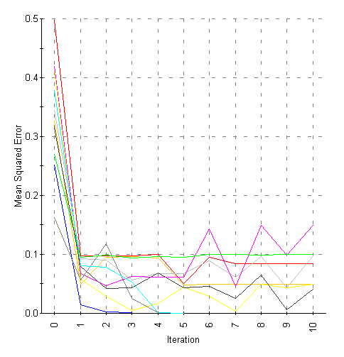
Figure 7: MSE for training a committee of ten neural networks on 104
channels selected by F-test
As can be seen in the
figure there is some over-training apparent in several networks.
However, experience has shown that moderate over-training on the
validation set is acceptable for small datasets, because the odds are
good that there is a significant difference between the samples
represented in the validation set for each network and the samples it
is trained on. This is not a flaw in the architecture, but a
reflection of the unfortunate and immutable fact that neural networks
require improbably large training sets if they are to be used in a
completely straightforward way—for reasonable sized training
sets a degree of insight and interpretation into their quality
measures is required.
To investigate the source
of overtraining, GeneLinkerTM Platinum includes a “pocket
algorithm” option for neural network training. This saves
(“pockets”) the network parameters that produce the best
performance on the validation set for each network, preventing
overtraining. If the overtraining is due to unrepresentative
validation sets the pocket algorithm will result in poorer
classifier performance on the whole dataset.
In this case, using the
pocket algorithm produces a similar level of performance, as does
cutting off training at 5 iterations rather than 10.
Testing the trained
committee of neural networks on the 30% of the data held out for
testing gives an error rate of 5 – 10%, depending on how
unknowns are counted. If an “unknown” classification is
counted as an error the typical accuracy is 91%, if unknowns are
excluded from the ratio then 95 – 96% accuracy is achievable.
While it is difficult to
improve the quality of discrimination, it is easy to reduce the
number of channels required to reach 95% discrimination accuracy.
Running Principle Component Analysis on the 104 channels identified
as significant by the by F-test shows that most of the between-group
variation is due to the first principle component, and there is a
small group of channels that accounts for most of the power in that
component.
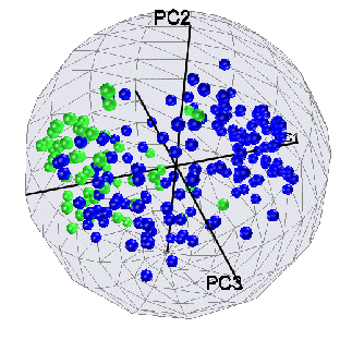
Figure 8: 3D PCA plot of 104 channels from F-test. Group D is green,
Group ABC is blue. Note that most of the D/ABC difference is
accounted for by PC1.
To reduce the number of
channels the PCA loadings are exported and re-imported into
GeneLinker as a new data table after editing the exported file to
remove all but the top five components. They are then
ranged-filtered to select the channels that have the largest
variation between components. This selects channels that account for
most of the variation in the data, and because the channels have
already been filtered to select those that vary significantly between
groups, this selects channels that vary most between groups. This
reduces the number of channels to 17, which produces perfect
performance on the training data after the elimination of 5 unknowns.
However, the performance on the held-out test data is not good:
only 88% correct classification after the elimination of unknowns.
The Kruskal-Wallis test is
a non-parametric version of the F-test, and produced similar results
on the un-normalized data to those of the F-test on the normalized
data.
To achieved better
discrimination the more powerful feature selectors available in
GeneLinker Platinum were brought into play: IBIS and SLAM. IBIS
(Integrated Bayesian Inference System) performs an exhaustive search
for single genes and pairs of genes that vary significantly between
classes using linear, quadratic or uniform Gaussian discriminant
analysis. SLAM performs a fast heuristic search for ntuples of genes
whose discretized levels of expression co-vary within a class
significantly more often than would be expected by chance.
For a dataset of moderate
size running IBIS on pairs of genes with QDA (quadratic discriminant
analysis) produces hundreds of discriminators with better than 80%
accuracy. Taking the top 97 genes from these gives a set of features
that with a four-hidden-node network gives 99% accuracy on the test
data with 3% unknowns.
Once a reasonable level of
discrimination has been achieved with a feature set of moderate size,
the next challenge is to reduce the number of features until the
minimal number has been found. This was done using a binary search
strategy: halving the number of features at each step. The results
are shown in Table 1.
The classification
accuracy is not a sensitive function of the number of features.
However, the best accuracy was achieved at 50 features (channels).
Larger numbers of channels perform less well due to noisier,
less-relevant data being included in the training process. Smaller
numbers of channels perform less well due to the absence of relevant
information.
The best performance is
very good: 99% correct classification on the held-out test data,
with only 1% (2 samples) not able to be classified. If unknowns are
(pessimistically) counted as misclassifications, this is still better
than 97% accuracy.
|
Fts.
|
Hidden Nodes
|
Training Accuracy
|
Training Unknowns
|
Test Accuracy
|
Test Unknowns
|
|
97
|
2
|
195/197 (99%)
|
5/202 (2.5%)
|
96/98 (98%)
|
6/104 (6%)
|
|
97
|
3
|
200/200 (100%)
|
2/202 (1.5%)
|
100/102 (98%)
|
2/104 (2%)
|
|
97
|
4
|
198/198 (100%)
|
4/202 (2%)
|
100/101 (99%)
|
3/104 (3%)
|
|
97
|
5
|
200/201 (99.5%)
|
1/202 (0.5%)
|
99/100 (99%)
|
4/104 (3%)
|
|
50
|
2
|
198/199 (99.5%)
|
3/202 (1.5%)
|
101/102 (99%)
|
2/104 (2%)
|
|
50
|
3
|
198/199 (99.5%)
|
3/202 (1.5%)
|
97/98 (99%)
|
6/104 (6%)
|
|
50
|
4
|
201/202 (99.5%)
|
0/202 (0%)
|
101/102 (99%)
|
2/104 (2%)
|
|
50
|
5
|
199/200 (99.5%)
|
2/202 (1%)
|
100/101 (99%)
|
3/104 (3%)
|
|
25
|
2
|
196/197 (99.5%)
|
5/202 (2.5%)
|
97/101 (96%)
|
3/104 (3%)
|
|
25
|
3
|
196/197 (99.5%)
|
5/202 (2.5%)
|
96/97 (99%)
|
7/104 (7%)
|
|
25
|
4
|
198/200 (99%)
|
2/202 (0.5%)
|
97/100 (97%)
|
4/104 (4%)
|
|
25
|
5
|
200/201 (99.5%)
|
1/202 (0.5%)
|
97/102 (95%)
|
2/104 (2%)
|
|
25
|
6
|
2/192 (99%)
|
10/202 (5%)
|
93/95 (98%)
|
9/104 (9%)
|
Table 1: Training and test accuracy of various feature sets selected
by the IBIS algorithm, as a function of the number of hidden neural
network nodes. The training set has 202 samples, the test set 104.
Only one network was trained for each configuration.
To explore improvements to
the accuracy to classification, SLAM was run on the log10-normalized
data for 5,000,000 iterations. This took several hours (dual 1GHz
desktop machine.)
Of the top 25 SLAM
channels, 11 differ from those found by IBIS. This illustrates the
value of the multiple approaches available in GeneLinker—the
SLAM-found channels are implicated in more complex protein-protein
interactions than the binary interactions that IBIS is sensitive to.
On the other hand, the signals that SLAM detects are often more
subtle and weaker than the pair-wise IBIS channels.
The SLAM-found channels
are not as good predictors as those found by IBIS. The best neural
network committee trained on the top 25 SLAM-found channels gives
only 95% correct classification with 6% unknowns. Interestingly,
they fail on a different set of samples than the top 25 IBIS channel
predictors do. This is a further illustration of the value of
multiple approaches—when the biological context is known, the
role of different feature sets can be interpreted to understand what
aspects of the biology they are sensitive to, rather than just
blindly selecting based on raw statistical significance, as is done
here.
The combined 36 unique
channels (11 from SLAM, 14 shared, 11 from IBIS) do not do
significantly better than the best 25 channels from IBIS alone.
The best 50 IBIS channels
are included in the appendix, along with their classifications of the
blinded test data included with the dataset using several committees
of neural networks trained on those channels.
Classification of Blinded Data
Classifying the blinded
data with the best neural network committee produces a higher than
expected proportion of unknowns: 6/60 (10%). This suggests that the
population for the blinded data may be slightly different from that
of the training data. A comparison of histograms adds a certain
amount of credence to this suggestion, as shown in Figure 9.
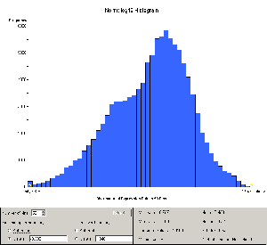
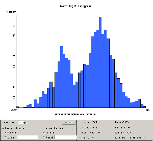
Figure 9: Comparison of histograms after negative value removal and
log10 normalization for training data and blinded test data. The
x-axis scales are identical in the two plots. While the
distributions are similar, there are clear and significant
differences
As a cross-check, several
other classifiers were run on the blinded data. In particular,
classifiers trained on the top 50 IBIS-selected channels with 2, 3, 4
and 5 hidden nodes were run. As shown in the appendix, in all but
one case (sample 14) at least one classifier was able to make a call.
In two cases (samples 22 and 53) only one classifier was able to
make a call. In all cases where more than one classifier was able to
make a call, there was complete agreement between them.
Appendix
Table 1A: Classification
of blinded samples based on top 50 IBIS channels. Note that in the
57 cases out of 60 where more than one classifier makes a call,
there is perfect agreement between the classifiers. Note that only
one sample cannot be classified at all.
|
Sample
|
2 Hidden
|
3 Hidden
|
4 Hidden
|
5 Hidden
|
Call
|
|
1
|
ABC
|
ABC
|
ABC
|
ABC
|
ABC
|
|
2
|
ABC
|
ABC
|
ABC
|
ABC
|
ABC
|
|
3
|
ABC
|
ABC
|
ABC
|
ABC
|
ABC
|
|
4
|
D
|
Unknown
|
D
|
D
|
D
|
|
5
|
Unknown
|
ABC
|
ABC
|
Unknown
|
ABC
|
|
6
|
ABC
|
ABC
|
ABC
|
ABC
|
ABC
|
|
7
|
ABC
|
ABC
|
ABC
|
ABC
|
ABC
|
|
8
|
ABC
|
ABC
|
ABC
|
ABC
|
ABC
|
|
9
|
ABC
|
ABC
|
ABC
|
ABC
|
ABC
|
|
10
|
ABC
|
ABC
|
ABC
|
ABC
|
ABC
|
|
11
|
D
|
D
|
D
|
D
|
D
|
|
12
|
D
|
D
|
D
|
D
|
D
|
|
13
|
D
|
D
|
D
|
D
|
D
|
|
14
|
Unknown
|
Unknown
|
Unknown
|
Unknown
|
Unknown
|
|
15
|
D
|
D
|
D
|
D
|
D
|
|
16
|
D
|
D
|
D
|
D
|
D
|
|
17
|
D
|
Unknown
|
Unknown
|
D
|
D
|
|
18
|
D
|
D
|
D
|
D
|
D
|
|
19
|
D
|
D
|
D
|
D
|
D
|
|
20
|
D
|
D
|
D
|
D
|
D
|
|
21
|
ABC
|
ABC
|
ABC
|
Unknown
|
ABC
|
|
22
|
Unknown
|
Unknown
|
Unknown
|
D
|
D
|
|
23
|
ABC
|
ABC
|
ABC
|
ABC
|
ABC
|
|
24
|
ABC
|
ABC
|
ABC
|
ABC
|
ABC
|
|
25
|
ABC
|
ABC
|
ABC
|
ABC
|
ABC
|
|
26
|
ABC
|
ABC
|
ABC
|
ABC
|
ABC
|
|
27
|
ABC
|
ABC
|
ABC
|
ABC
|
ABC
|
|
28
|
ABC
|
ABC
|
ABC
|
ABC
|
ABC
|
|
29
|
ABC
|
ABC
|
ABC
|
ABC
|
ABC
|
|
30
|
ABC
|
ABC
|
ABC
|
ABC
|
ABC
|
|
31
|
ABC
|
ABC
|
ABC
|
ABC
|
ABC
|
|
32
|
ABC
|
ABC
|
ABC
|
ABC
|
ABC
|
|
33
|
ABC
|
ABC
|
ABC
|
ABC
|
ABC
|
|
34
|
ABC
|
ABC
|
ABC
|
ABC
|
ABC
|
|
35
|
ABC
|
ABC
|
ABC
|
ABC
|
ABC
|
|
36
|
D
|
D
|
D
|
D
|
D
|
|
37
|
D
|
D
|
D
|
D
|
D
|
|
38
|
D
|
D
|
D
|
D
|
D
|
|
39
|
D
|
D
|
D
|
D
|
D
|
|
40
|
D
|
D
|
D
|
D
|
D
|
|
41
|
ABC
|
ABC
|
ABC
|
ABC
|
ABC
|
|
42
|
ABC
|
ABC
|
ABC
|
ABC
|
ABC
|
|
43
|
ABC
|
ABC
|
ABC
|
ABC
|
ABC
|
|
44
|
ABC
|
ABC
|
ABC
|
Unknown
|
ABC
|
|
45
|
D
|
D
|
D
|
D
|
D
|
|
46
|
D
|
D
|
D
|
D
|
D
|
|
47
|
ABC
|
ABC
|
ABC
|
ABC
|
ABC
|
|
48
|
ABC
|
ABC
|
ABC
|
ABC
|
ABC
|
|
49
|
ABC
|
ABC
|
ABC
|
ABC
|
ABC
|
|
50
|
ABC
|
ABC
|
ABC
|
ABC
|
ABC
|
|
51
|
ABC
|
ABC
|
ABC
|
ABC
|
ABC
|
|
52
|
ABC
|
ABC
|
ABC
|
ABC
|
ABC
|
|
53
|
Unknown
|
ABC
|
Unknown
|
Unknown
|
ABC
|
|
54
|
ABC
|
ABC
|
ABC
|
Unknown
|
ABC
|
|
55
|
ABC
|
ABC
|
ABC
|
ABC
|
ABC
|
|
56
|
D
|
D
|
D
|
D
|
D
|
|
57
|
D
|
D
|
D
|
D
|
D
|
|
58
|
D
|
Unknown
|
Unknown
|
D
|
D
|
|
59
|
D
|
Unknown
|
Unknown
|
D
|
D
|
|
60
|
D
|
D
|
D
|
D
|
D
|

