An Introduction to Classification: Feature Selection

This document introduces the topic of classification, presents the concepts of features and feature identification, and ultimately discusses the problem that GeneLinker™ Platinum solves: finding non-linearly predictive features that can be used to classify gene expression data. Many examples, some very simple, are used clarify subtle and sometimes difficult concepts.

Classification

There are several types of classification:

Categorical classification is also called nominal classification because it classifies an entity in terms of the name of the class it belongs to. This is the type of classification we focus on in this document.

Features

If we think for a minute about how we classify common everyday objects such as people and cars, it's pretty clear that we are using features of those objects to do the job. People have legs, that's a feature that cars don't have. Cars have wheels, that's a feature that people don't have. By selecting the appropriate set of features, we can do a good job of classification.

To make this kind of feature-based classification work, we need to have some knowledge of what features make good predictors of class membership for the classes we are trying to distinguish. For example, having wheels or not distinguishes people from cars, but doesn't distinguish cars from trains. These are two different classification tasks. Depending on the classification task we are facing, different features or sets of features may be important, and knowing how we arrive at our knowledge of which features are useful to which task is essential.

Learning

The general process by which we gain knowledge of which features matter in a given discrimination task is called learning. For those of us who are parents, one example of this type of learning (feature selection) involves teaching our children about types of animals. We (endlessly) point to animals and say words like dog or cat or horse. We don't generally give our children a feature list that a biologist might use to define Canis familiaris or Felis catus. Instead, we present examples and expect our children to figure out for themselves what the important features are. And when they make a correct guess about an animal (a correct classification or prediction), we give copious amounts of positive feedback.

This procedure is called supervised learning. We present our children or our computer programs with examples and tell them what category each example belongs to, so they learn under our supervision. This is in contrast to unsupervised learning. In unsupervised learning objects are grouped together based on perceptions of similarity (or more properly, relative lack of difference) without anything more to go on. While unsupervised learning is indispensable, supervised learning has a substantial advantage over unsupervised learning.

In particular, supervised learning allows us to take advantage of our own knowledge about the classification problem we are trying to solve. Instead of just letting the algorithm work out for itself what the classes should be, we can tell it what we know about the classes: how many there are and what examples of each one look like. The supervised learning algorithm’s job is then to find the features in the examples that are most useful in predicting the classes.

The clustering algorithms in GeneLinker™ Gold are examples of unsupervised learning algorithms. The classification workflows of GeneLinker™ Platinum are examples of supervised learning algorithms. They are more complex than clustering, and sometimes more frustrating due to their additional complexity, but they have considerable advantages.

The classification process with supervised learning always involves two steps:

1. Training (with assessment) – this is where we discover what features are useful for classification by looking at many pre-classified examples.

2. Classification (with assessment) – this is where we look at new examples and assign them to classes based on the features we have learned about during training.

This process isn’t perfect, particularly if the number of examples used in training is small. A difficult problem is how to handle objects that don't fall into any of the classes we know about. There is a tendency to categorize them as belonging to one of the classes we do know about, even if the fit is rather poor. For example, upon seeing a horse for the first time, my son announced, 'Look! Big dog!' GeneLinker™ Platinum's classification algorithms are capable of making this kind of error.

The Problem

The problem that GeneLinker™ Platinum is the solution to is the classification problem, which is:

1. How do we find a set of features that is a good predictor of what class a sample belongs to?

2. Having found a good set of features, how do we use it to predict what classes new samples belong to?

The first part of the classification problem, which is by far the hardest, is solved by the Sub-Linear Association Mining (SLAM™) and other Predictive Patterns Software Inc. proprietary data mining algorithms. The second is solved by our committee of artificial neural networks (ANNs) or committee of support vector machines (SVMs).

Feature Selection

Features in Data

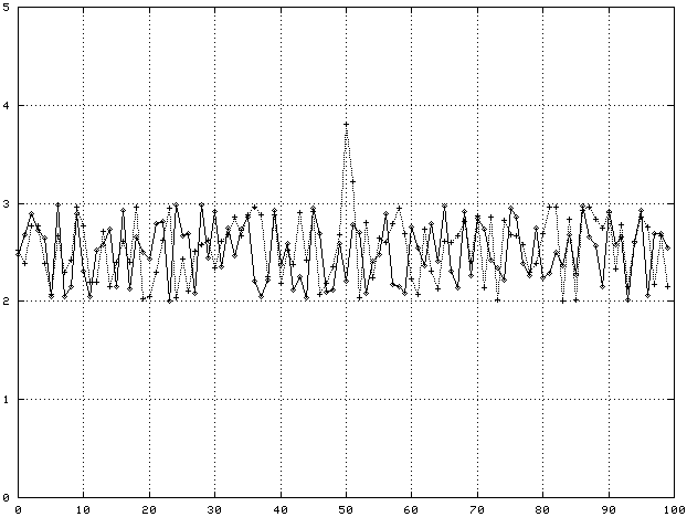
Before getting into feature selection in more detail, it's worth making concrete what is meant by a feature in gene expression data. The figure below shows two genes with 100 samples each. One gene, call it Gene A, clearly has an enhanced expression value around sample 50. This expression level ‘bump’ is a feature. If every gene expression profile from tissues of the same class showed the same bump, this feature would be a good predictor of what tissue class a new sample of tissue belonged to.

Suppose we observed the following data:

In this case, Gene A has a feature, an enhanced expression level for sample 50, that is a good predictor of which class (Normal or Cancer) a tissue belongs to. Gene B has no such feature, its average expression level at sample 50 is independent of tissue class.

Probability

So far, it may seem as though a nice clean distinction between features that distinguish classes clearly and those that don't always exists. In fact, this is rarely the case. Most of the time all we see is an enhanced correlation between a feature and a class.

For example, tall people tend to be stronger than short people. There are several reasons for this: tall people have longer arms and legs, which gives their muscles more mechanical advantage; tall people tend to have bigger muscles, simply because they are bigger people; and tall people tend to be men, who have higher testosterone levels, which helps them build more muscle. The fact remains, however, that some short women can lift more weight than some tall men. So if we were to try to classify people into two groups, ‘strong’ and ‘weak’, without actually measuring how much they can lift, height might be one feature we would use as a predictor. But, it couldn't be the only one if we wanted our classification to be highly reliable.

If a single feature is not a good class predictor on its own, the alternative is to look for one or more sets of features that together make a good predictor of what class an object falls into. For example, neither height nor weight are particularly good predictors of obesity; but taken together, they predict it fairly well.

Linearly Predictive Features

The tissue data above is an example of a linearly predictive feature. That is, when the expression level of gene A goes up at sample 50, the probability that the tissue is normal goes up too. This can be expressed mathematically by the linear equation:

P(normal) = k*XA

where P(normal) is the probability the tissue is Normal, XA is the expression level of gene A, and k is a constant that depends on the specifics of the data. The expression level of gene A at sample 50 is also a linear predictor of the probability that the tissue is a cancer:

P(cancer) = 1 - P(normal) = 1 - k*XA

In this case, the linear relationship is inverted: the higher the expression level of gene A at sample 50, the lower the probability of the tissue being in the cancer class.

Combinations of Linearly Predictive Features

The wonderful thing about linearly predictive features is that they combine linearly. This means that they obey the familiar laws of arithmetic when they are combined: literally, 2 + 2 = 4 for linearly predictive features. This is not the case for non-linearly predictive features. Not only does this make linearly predictive features easy to understand, it makes the algorithmic mathematical problem of finding them tractable.

For example, consider the example of height and weight as predictors of obesity. Although not strictly linear, they are approximately so. They are in fact an example of monotonic predictors - as they increase or decrease, the probability of a sample being in a particular class increases or decreases as well. It is never the case, for example, that a light person is more likely to be obese than a heavy person. The heavier you are, the more likely you are to be obese, no matter how tall you are. Monotonic predictors can usually be approximated by linear predictors, at least over a limited range, as shown in the following figure.

Biologically, saturation is a common cause of non-linear but still monotonic behavior. For example, if a given enzyme binds to a particular receptor, more enzyme will result in a larger effect up to the point where all the receptors are already bound to enzyme molecules. At that point, the system is saturated and the effect won't increase no matter how much more of the enzyme is added.

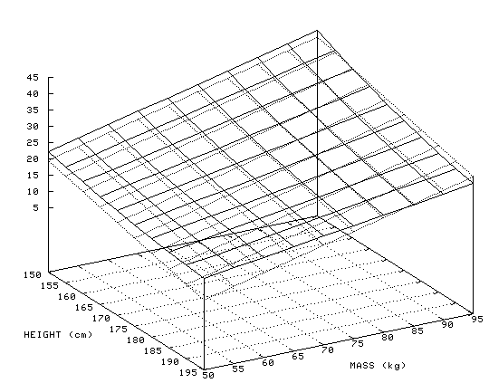
The figure below shows body mass index (BMI) as a function of height and weight. A BMI of greater than 25 indicates a person who is overweight, and greater than 29 indicates a person who is obese. The dark gray surface is BMI, the light gray surface is a linear approximation to BMI:

BMI(Height, Weight) = 40 - 0.29*Height + 0.46*Weight

As can be seen from the size of the coefficients, height has a smaller influence on BMI than weight does, but neither of them has such a dramatic influence that it would be possible to ignore the other. The linear combination of features, high weight and low height, or very high weight and high height, is required to classify a person as obese.

Mathematically, combinations of linearly predictive features are easy to extract from even fairly small sets of examples. This is because of the fact that linearly mathematical problems are invertible: in one-dimensional terms, if we know Y = k*X, then we also know k = Y/X, which gives us the constant that relates the feature to the probability of being in a given class. This process can be generalized to combinations of features as well, ultimately meaning that there are tedious but straightforward deterministic mathematical algorithms for extracting linear combinations of features that have good predictive power. One such algorithm is principal component analysis (PCA).

Non-linearly Predictive Features

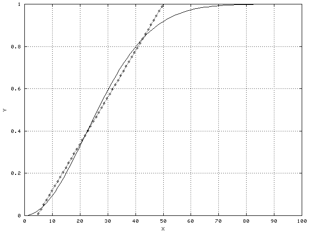
Not all classes have linearly predictive features: that is, the probability of an object belonging to a given class cannot be written as a linear function of some set of features. For example, consider weight as a predictor of vehicle class. In particular, consider distinguishing cars from aircraft by weight. If a vehicle is very light, it is probably an air-craft. Most small planes weigh quite a bit less than a car. However, if a vehicle is in the range of one to two thousand pounds, it's probably a car, and if it's much heavier than that it's probably a light jet or larger.

In this case, unlike the monotonic, non-linear case, it is practically impossible to approximate the non-linear features with a linear function over a small range. The probability that a vehicle is a car as a function of weight looks something like this:

As this is not a straight line, linear approximations don’t apply.

Combinations of Non-linearly Predictive Features

Combinations of non-linearly predictive features are the most general case a feature selector has to handle. Many biological classification problems can only be solved by such combinations, and unfortunately, the problem of finding a good set of non-linearly predictive features is very nearly intractable.

The reason for this is that unlike linear problems, non-linear problems cannot be inverted. There is no way of turning the equation around and extracting the parameters (the equivalents of the linear constants) that will give us good predictions. This means that the only way we have of finding the combinations of features that give us good predictive power is to search for them, checking combinations of features one by one and trying to figure out what combination gives us the best ability to classify objects into different categories of interest.

The Combinatoric Explosion

The simplest way to search for combinations of features that give us good predictive power is to start by looking at features one at a time, and trying to find ones that are predictive of the classes we are interested in. But we've already seen that sometimes features that have little or no predictive power on their own, like height for obesity, but are very powerful predictors when combined with other features. Therefore, we have to search not only individual features, but also combinations.

If we have ten genes and look at all pairs, we have 10^2 = 100 possible combinations. If we look at all possible triples we have 10^3 = 1000 possible combinations, and so on for quads and quintuplets. For a typical 10,000 gene Affymetrix chip, the number of pairs we have to search through is a hundred million, the number of triples is a trillion, and the number of quads and quintuplets is astronomical.

This dramatic increase in the number of possible combinations as the number of samples goes up is known as the combinatoric explosion, and it is the source of intractability in non-linear combinatoric feature selection. Non-linearity forces us to use a search technique to find the features that give us the best classification of our objects of interest, and the combinatoric explosion makes simple exhaustive search impossible on all but the smallest datasets.

An example of a non-linear combinatoric problem we're all familiar with is time management. At any given time there are dozens of things we might plausibly be doing. Time management is essentially a problem of task categorization. There are two classes of task: ‘critical’, which is the one we should be doing right now; and ‘non-critical’, which is everything else.

Each task that faces us has many possible features we might use to categorize it as ‘critical’: how important is it to our long-term goals, to our short-term goals? How much fun would it be? How important is it to our boss or our spouse or our children or our friends? How long have we been putting it off? Do we need to do it to fulfill some condition on another task we need to get done? And so on. Even selecting a few good features out of this short list to let us classify tasks is a hard problem.

People often focus on the single feature that seems to have the most predictive power on its own. They may use features such as ‘serves my short-term goals’ or ‘makes my spouse or boss happy’ to identify ‘critical’ tasks. They forget that even if we are highly focused on productivity, it's still the case that sometimes the most important task is to go lie on the beach and relax. This is a highly non-linear effect. By itself, ‘makes me feel good’ is not a good predictor of a whether or not a task is ‘critical’, but taken in combination with other task features, it becomes a valuable member of the most predictive feature set.

The classification problem is hard because features have non-linear effects, and combine together in non-linear ways. This means that there is no way to select features that have good classifying power without doing some kind of search through combinations of features. Because the number of possible combinations of features is impossibly large, simply searching through all feature combinations is not practical.

The Platinum Solution

In the gene expression analysis arena, the solution to this problem is the SLAM™ algorithm embodied in GeneLinker™ Platinum. This algorithm uses intelligent heuristics to guide the search for combinations of features with high predictive value toward a small subset of combinations that have a good chance of correctly classifying all the examples presented to the algorithm. Once a feature set has been identified by SLAM, it can be used to train a committee of artificial neural networks or support vector machines that can be used to classify new examples. This combined workflow of feature selection, classifier training, and applying the trained classifier to new samples is the core of GeneLinker™ Platinum’s powerful classification solution.